Eoghan O'Meara
New Member
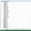
I have recently upgraded from Office 2010 to Office 2013. I created a new pivot tablem and I have noticed that when I now filter my pivot table results, instead of hiding rows, it seems to remove them e.g. instead of displaying results with their original row number before the filter, it recalculates the row numbers to run contiguously. (See sample below) *Option 1* However, what I want is for it maintain the original row number of the data (as in the sample screenshot below). *Option 2*

I've played around with this most of this morning, and it seems to be quite subjective in terms of which approach it takes (roughly 80% of the time it will return results in the style of sample 1, the remainder in the style of sample 2). This is the case even when the steps are exactly the same. It's worth noting that my experience is the same irrespective of whether I:
- use the row label filters
- apply a filter by selecting the title row when highlighting the cell to the right of the pivot table (See image)

- use the label filter or value options in the row labal
Can someone advise what the cause is and how I can ensure to get Option 2 each time. Please note, I'm not looking for an alternate solution here, I'm conscious of loads of formula based solutions that I could ultimately use to get to the point I want with this data, but owing to the volume and complexity of the data, it really is important for me that the original row numbers are maintained.
 However, what I want is for it maintain the original row number of the data (as in the sample screenshot below). *Option 2*
I've played around with this most of this morning, and it seems to be quite subjective in terms of which approach it takes (roughly 80% of the time it will return results in the style of sample 1, the remainder in the style of sample 2). This is the case even when the steps are exactly the same. It's worth noting that my experience is the same irrespective of whether I:
- use the row label filters
- apply a filter by selecting the title row when highlighting the cell to the right of the pivot table (See image)

- use the label filter or value options in the row labal
Can someone advise what the cause is and how I can ensure to get Option 2 each time. Please note, I'm not looking for an alternate solution here, I'm conscious of loads of formula based solutions that I could ultimately use to get to the point I want with this data, but owing to the volume and complexity of the data, it really is important for me that the original row numbers are maintained.

